필기체를 구분하는 분류 ANN

 

ann_mnist_cl.py

0.00MB

1단계 : 케라스 패키지에서 2가지 모듈을 불러옴

#분류 ANN을 위한 인공지능 모델 구현
from keras import layers, models

layers는 각 계층을 만드는 모듈

models는 각 layer들을 연결하여 신경망 모델을 만든 후, 컴파일하고 학습시키는 역할, 평가도 포함

 

객체지향 방식을 지원하는 케라스는 models.Model 객체에서 compile(), fit(), predict(), evaludate() 등 딥러닝 처리 함수 대부분을 제공 

 

Nin : 입력계층의 노드 수

Nh : 은닉 계층의 노드 수

number_of_class : 출력값이 가질 클래스 수

Nout : 출력 노드 수

 

 

2단계 : ANN 모델을 분산 방식으로 구현, 모델 구현에는 함수형 방식을 사용

x = layers.Input(shape=(Nin,))

입력 계층을 layers.Input() 함수로 정의

h = layers.Activation('relu')(layers.Dense(Nh)(x))

은닉 계층을 layers.Dense() 함수로 지정

x를 입력으로 받아들이도록 layers.Dense(Nh)(x)로 지정

활성화 함수로는 layers.Activation('relu') 로 지정했는데, ReLU는 활성화 함수로 f(x) = max(x,0)과 같음

y = layers.Activation('softmax')(layers.Dense(Nout)(h))

출력 계층을 구현

분류의 경우에는 활성화 함수로 소프트맥스 연산을 사용

model = models.Model(x,y)
model.compile(loss='categorical_crossentropy',
              optimizer='adam', metrics=['accuracy'])

인공지능 모델을 구현

파이썬은 스크립트 언어이기에 별 다른 컴파일이 없어도 실행 가능

컴파일 과정에서 loss는 손실 함수를 지정하는 아규먼트, optimizer은 최적화 함수를 지정, metrics는 학습이나 예측이 진행될 때 성능 검증을 위해 손실뿐 아니라 정확도 즉, accuracy를 측정

 

 

3단계 : 연쇄 방식 모델링을 포함하는 함수형 구현

model = models.Sequential()

분산 방식과 다르게 모델을 먼저 설정

연쇄 방식은 모델 구조를 정의하기 전에 Sequential() 함수로 모델을 초기화해야 함

model.add(layers.Dense(Nh, activation='relu', input_shape=(Nin,)))
model.add(layers.Dense(Nout, activation='softmax'))

첫번째 add에서 입력 계층과 은닉 계층 형태가 동시에 정해짐

은닉 계층의 노드들은 ReLU를 활설화 함수로 사용

활성화 함수로 소프트맥스 연산을 사용

 

연쇄 방식의 장점 ?

추가되는 계층을 기술할 때 간편하게 기술 가능

- add()를 이용해 연속되는 계층을 계속 더해주면 됨

 

+ 복잡한 인공신경망을 기술하는 부분은 연쇄형 모델링만으로 구현이 힘든 경우가 있음. 이 같은 경우에는 분산 방식 모델링을 사용

 

4단계 : 분산 방식 모델링을 포함하는 객체지향형 구현

class ANN_models_class(models.Model):
    def __init__(self, Nin, Nh, Nout):

클래스를 만들고 models.Model로부터 특성을 상속 받고 클래스의 초기화 함수를 정의

models.Model은 신경망에서 사용하는 학습, 예측, 평가와 같은 다양한 함수 제공

hidden = layers.Dense(Nh)

신경망 모델에 사용할 계층 정의

output = layers.Dense(Nout)

노드 수가 Nout 개인 출력 계층을 정의

relu = layers.Activation('relu')
softmax = layers.Activation('softmax')

비선형을 넣어주는 activation 함수를 정의

relu와 softmax는 계산 모듈이므로 한 번 정의해두면 모델 내에서 여러번 사용 가능

ReLU : 0보다 큰 수는 그대로 출력, 0보다 더 작은 수는 0으로 출력

분류의 경우, 출력 노드의 활성화 함수로 소프트맥스 연산을 사용

super().__init__(x,y)

상속받은 부모 클래스의 초기화를 진행

model = ANN_models_class(Nin, Nh, Nout)

모델을 사용하기 위해 인스턴스를 생성

 

+ 이번 ANN은 은닉 계층이 하나이기에 hidden을 하나로 정의하였는데,

만일 은닉 계층이 n개 라면 반복문을 사용해서 생성 가능(아래 코드 예시)

hidden_l = []
for n in Nh_l:
	hidden_l.append(layers.Dense(n))

 

객체지향 방식의 장점 ?

일반 사용자의 경우 전문가가 만든 인공지능 모델을 객체로 불러 쉽게 활용 가능(코드의 재사용성)

 

 

5단계 : 연쇄 방식 모델링을 포함하는 객체지향형 구현

class ANN_seq_class(models.Sequential):
    def __init__(self, Nin, Nh, Nout):
        super().__init__()

models.Sequential에서 상속 받음

부모 클래스의 초기화 함수를 자신의 초기화 함수 가장 앞에서 호출

self.add(layers.Dense(Nh, activation='relu', input_shape=(Nin,)))

입력 계층을 별도로 정의하지 않고 은닉계층부터 추가

self.add(layers.Dense(Nout, activation='softmax'))

출력계층을 정의

 

6단계 : 분류 ANN에 사용할 데이터 불러오기

 

데이터를 불러오고 전처리 하는 과정 ?

1. 데이터 처리에 사용할 패키지 임포트

2. 데이터 불러오기

3. 출력값 변수를 이진 벡터 형태로 바꾸기

4. 이미지를 나타내는 아규먼트를 1차원 벡처 형태로 바꾸기

5. ANN을 위해 입력값들을 정규화(regularization)하기

 

import numpy as np
from keras import datasets
from keras.utils import np_utils

넘파이 라이브러리는 reshape() 멤버 함수를, 케라스의 datasets 라이브러리는 mnist() 함수를, keras.utils의 np.utils 라이브러리는 to_categorical() 함수를 사용하고자 라이브러리를 import

 

(X_train, y_train), (X_test, y_test) = datasets.mnist.load_data()

MNIST 데이터를 불러와서 변수에 저장

학습에 사용하는 데이터는 _train으로 끝나는 변수에 저장, 성능 평가에 사용할 데이터는 _test으로 끝나는 변수에 저장

 

딥러닝에 사용되는 데이터는 학습(training), 검증(validation), 평가(test) 데이터 3가지로 분류

학습 데이터는 모델을 학습하는데 사용되는 데이터

검증 데이터는 학습이 진행되는 동안 성능을 검증하는데 사용되는 데이터

평가 데이터는 학습을 마치고 나서 모델의 성능을 최종적으로 평가하는데 사용하는 데이터

Y_train = np_utils.to_categorical(y_train)
Y_test = np_utils.to_categorical(y_test)

0부터 9가지의 숫자로 구성된 출력값을 0과 1로 표현되는 벡터 10개로 교체

ANN을 이용한 분류 작업 시 정수보다 이전 벡터로 출력 변수를 구성하는 것이 효율적

L, W, H = X_train.shape
X_train = X_train.reshape(-1, W*H)
X_test = X_test.reshape(-1, W*H)

(x, y) 축에 대한 픽셀 정보가 들어 있는 3차원 데이터인 실제 학습 및 평가용 이미지를 2차원으로 조정

shape에는 2D 이미지 데이터를 저장하는 저장소의 규격이 들어가 있는데, 이를 ANN으로 학습하기위해서는 벡터 이미지 형태로 바꾸어야 되기에 reshape() 함수를 사용

-1는 행렬의 행을 자동으로 설정하게 만듬

X_train = X_train/255.0
X_test = X_test/255.0

0~ 255 사이의 정수로 구성된 입력값을 255로 나누어 0~ 1 사이의 실수로 바꾸어 아규먼트를 정규화

 

 

분류 ANN 학습 결과 그래프 구현

import matplotlib.pyplot as plt

그래프를 그리는 라이브러리 plt를 import

 

plt.plot() : 선 그리기

plt.title() : 그래프 제목 표시

plt.xlabel() : x축 이름 표시

plt.ylabel() : y축 이름 표시

plt.legend() : 각 라인의 표식 표시

def plot_loss(history):
    plt.plot(history.history['loss'])
    plt.plot(history.history['val_loss'])
    plt.title('Model Loss')
    plt.ylabel('Loss')
    plt.xlabel('Epoch')
    plt.legend(['Train', 'Validation'], loc=0)

손실을 그리는 함수

def plot_acc(history):
    plt.plot(history.history['accuracy'])
    plt.plot(history.history['val_accuracy'])
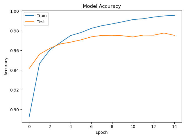
    plt.title('Model Accuracy')
    plt.ylabel('Accuracy')
    plt.xlabel('Epoch')
    plt.legend(['Train', 'Test'], loc=0)

정확도를 그리는 함수

 

 

7단계 : 분류 ANN 학습 및 성능 분석

def main():
    Nin = 784
    Nh = 100
    number_of_class = 10
    Nout = number_of_class
    model = ANN_seq_class(Nin, Nh, Nout)
    (X_train, Y_train), (X_test, Y_test) = Data_func()

모델의 인스턴스를 만들고 데이터를 불러옴

history = model.fit(X_train, Y_train, epochs=15,
                    batch_size=100, validation_split=0.2)

epochs : 반복할 횟수

batch_size : 데이터를 얼마씩 나눠서 넣을지 지정하는 값

validation_split : 전체 학습 데이터 중 성능 검증에 데이터를 얼마나 사용할지 결정하는 변수(0~1 사이의 수(ex. 0.2면 20%))

결과값

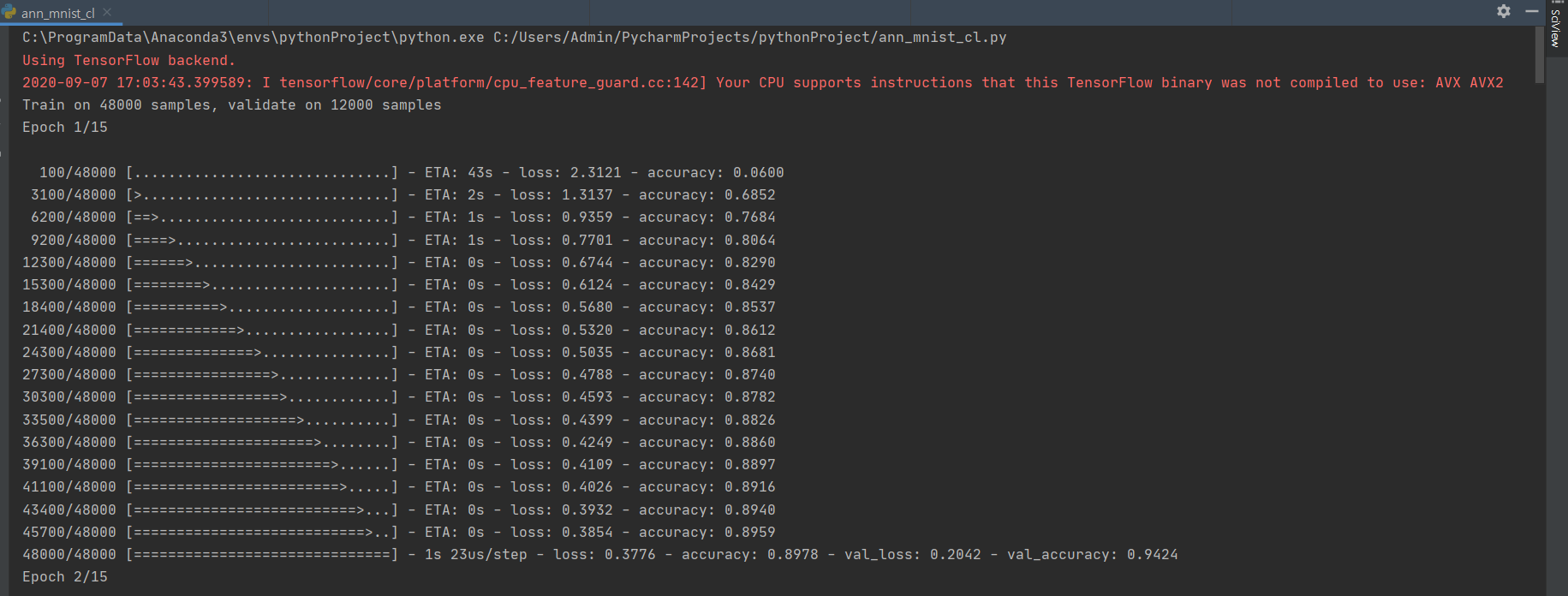
Train on 48000 samples, validate on 12000 samples : 학습에 주어진 샘플 60,000개중 48,000개가 실제 학습에 사용되고 12,000개가 검증에 사용

Epoch 1/15 : 15번의 반복 학습에서 첫 번째 단계 학습이 완료

1s : 학습에 걸린 시간이 1초

loss: 0.3776 : 손실이 0.3776, loss는 손실 함수로 구한 오류율

accuracy: 0.8978 : 정확도가 0.8978, 정확히 예측했을 경우 최댓값 1을 가짐

val_loss: 0.2042 - val_accuracy: 0.9424 : 검증 데이터로 측정한 손실과 정확도

 

perfomace_test = model.evaluate(X_test, Y_test, batch_size=100)
print('Test Loss and Accuracy - >', perfomace_test)

(X_test, Y_test)로 성능을 최종 평가

fit()함수와 같이 evaluate()에서도 batch_size 변수로 한번에 계산할 데이터 길이를 지정

ANN 학습 과정에서 손실 학습 곡선

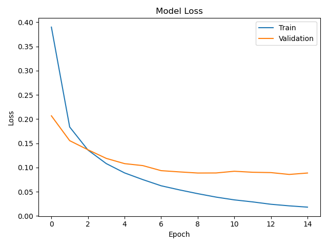
결론 : epoch가 4회 이상 넘어가면 학습 데이터로 구한 손실은 계속 줄어드는 반면 검증 데이터로 구한 손실은 거의 변하지 않고 뒤로 갈수록 오히려 약간 나빠진다. 설정한 ANN이 가지는 자유도에 비해 학습 데이터 수가 적거나 학습 방법에 한계가 있기 때문에 오는 과적합 현상이다. 이를 방지하기에는 학습을 조기에 끝내는 조기 종료나 모델에 사용된 파라미터 수를 줄이는 방법이 있다.

 

=> 학습 곡선을 모니터링하고 조기 종료 위치를 정하거나 인공신경망의 모델을 조정하는 것은 ANN의 최적화에 매우 중요

 

ANN 학습 과정에서 정확도 학습 곡선

 

 

전체 코드

#분류 ANN을 위한 인공지능 모델 구현
from keras import layers, models

# 분산 방식 모델링을 포함하는 함수형 구현
def ANN_models_func(Nin, Nh, Nout):
    x = layers.Input(shape=(Nin,))
    h = layers.Activation('relu')(layers.Dense(Nh)(x))
    y = layers.Activation('softmax')(layers.Dense(Nout)(h))
    model = models.Model(x,y)
    model.compile(loss='categorical_crossentropy',
                  optimizer='adam', metrics=['accuracy'])
    return model

# 연쇄 방식 모델링을 포함하는 함수형 구현
def ANN_seq_finc(Nin, Nh, Nout):
    model = models.Sequential()
    model.add(layers.Dense(Nh, activation='relu', input_shape=(Nin,)))
    model.add(layers.Dense(Nout, activation='softmax'))
    model.compile(loss='categorical_crossentropy',
                  optimizer='adam',
                  metrics=['accuracy'])
    return model

#분산 방식 모델링을 포함하는 객체지향형 구현
class ANN_models_class(models.Model):
    def __init__(self, Nin, Nh, Nout):
        hidden = layers.Dense(Nh)
        output = layers.Dense(Nout)
        relu = layers.Activation('relu')
        softmax = layers.Activation('softmax')

        x = layers.Input(shape=(Nin,))
        h = relu(hidden(x))
        y = softmax(output(h))

        super().__init__(x,y)
        self.compile(loss='categorical_crossentropy',
                     optimizer='adam',
                     metrics=['accuracy'])

# 연쇄 방식 모델링을 포함하는 객체지향형 구현
class ANN_seq_class(models.Sequential):
    def __init__(self, Nin, Nh, Nout):
        super().__init__()
        self.add(layers.Dense(Nh, activation='relu', input_shape=(Nin,)))
        self.add(layers.Dense(Nout, activation='softmax'))
        self.compile(loss='categorical_crossentropy',
                     optimizer='adam',
                     metrics=['accuracy'])

# 분류 ANN에 사용할 데이터 불러오기
import numpy as np
from keras import datasets
from keras.utils import np_utils

def Data_func():
    (X_train, y_train), (X_test, y_test) = datasets.mnist.load_data()

    Y_train = np_utils.to_categorical(y_train)
    Y_test = np_utils.to_categorical(y_test)

    L, W, H = X_train.shape
    X_train = X_train.reshape(-1, W*H)
    X_test = X_test.reshape(-1, W*H)

    X_train = X_train/255.0
    X_test = X_test/255.0

    return (X_train, Y_train), (X_test, Y_test)

# 분류 ANN 학습 결과 그래프 구현
import matplotlib.pyplot as plt

def plot_loss(history):
    plt.plot(history.history['loss'])
    plt.plot(history.history['val_loss'])
    plt.title('Model Loss')
    plt.ylabel('Loss')
    plt.xlabel('Epoch')
    plt.legend(['Train', 'Validation'], loc=0)

def plot_acc(history):
    plt.plot(history.history['accuracy'])
    plt.plot(history.history['val_accuracy'])
    plt.title('Model Accuracy')
    plt.ylabel('Accuracy')
    plt.xlabel('Epoch')
    plt.legend(['Train', 'Test'], loc=0)

# 분류 ANN 학습 및 성능 분석
def main():
    Nin = 784
    Nh = 100
    number_of_class = 10
    Nout = number_of_class

    model = ANN_seq_class(Nin, Nh, Nout)
    (X_train, Y_train), (X_test, Y_test) = Data_func()

    history = model.fit(X_train, Y_train, epochs=15,
                        batch_size=100, validation_split=0.2)
    perfomace_test = model.evaluate(X_test, Y_test, batch_size=100)
    print('Test Loss and Accuracy - >', perfomace_test)

    plot_loss(history)
    plt.show()
    plot_acc(history)
    plt.show()

if __name__ == '__main__':
    main()

 

 

reference ? 

한빛 미디어  / 코딩 셰프의 3분 딥러닝 케라스맛